Greetings, O dearest droogies! You've arrived at yet another look at how we live in a society, and why that's kinda neat. I'll do my best to keep it easier to understand than a big stick as I beat facts into your head, a Chiron guiding you through the river statis-Styx. Without further ado, let's take a deep dive into the thrilling (but not really) world of Union Density, GDP, and their tumultuous relationship. Buckle up, buttercup, and let's get this show on the road!
Setting the Scene:
Once upon a time and a half, our two protagonists, Union Density (y) and GDP (X), found themselves in the same dataset. The data was sourced from the International Labour Organization (ILO) and the World Happiness Report, which - let's be honest - is the only report we all really care about. And me, the daring data analysts, armed with curiosity from seeing a really bad take on twitter, and a flair for the dramatic, set out to answer the age-old question: "Is there a relationship between Union Density and GDP?"
The Plot Thickens:
After going through the long and tedious ordeal of data cleaning, checking distributions, and various visualizations, I got to the Pearson's correlation coefficient, the hero of our story.
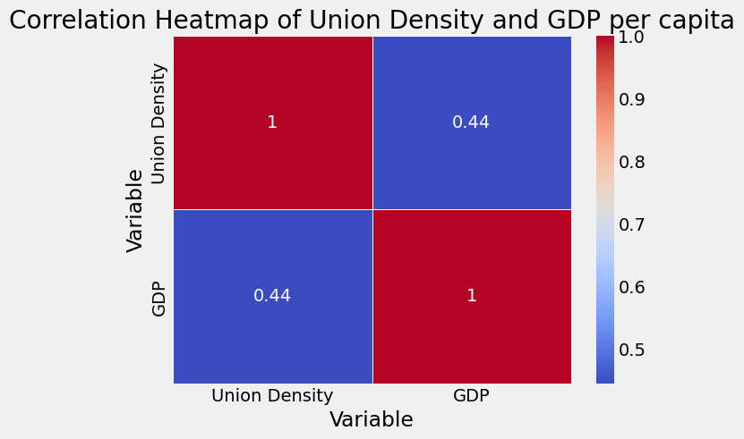
Basically, Pearson's correlation coefficient helps us see if two things are related and how they move together, whether they move in the same or opposite directions.
If it's close to 1, it means there's a strong positive relationship between the variables – as one goes up, so does the other. If it's close to -1, then you have a more see saw thing going on, one bounces up, the other goes down. If it's close to 0, it means there's little to no relationship between the variables – just like me and dad. :)
Running our little shreksperiment, a Pearson coefficient of 0.44422304265859053. For those of you not familiar with the thrilling world of correlation coefficients, the statistical value of 0.4442 suggests that there's some positive relationship between Union Density and GDP... But we're not done quite yet.
Now, the Pearson correlation coefficient measures the strength and direction of a relationship between two variables. It shows us how closely the variables are related and whether they move together or against each other. However, it can't tell us if the observed relationship could have happened by chance.
That's why we also use p value. The p value helps determine if the two variables are statistically significant, meaning they're unlikely to have occurred by chance. Typically, if the p value is less than a predetermined threshold (e.g., 0.05), we assume the relationship is statistically significant.
For us, the p value of 0.000765 shows that the likelihood of our observed correlation occurring by pure chance is super low (less than 0.1% even).
Pretty wizard, right? Now I'm sure every union worker is ready to pop champagne 🍾, but hold up. We gotta remember correlation doesn't equal causation, a mantra we should remember as we cry ourselves to sleep.
Plot thiccens:
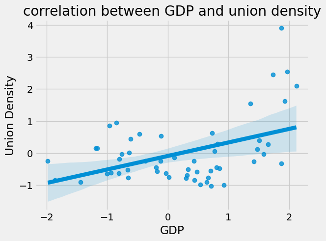
Why stop at a Pearson when everyone loves lijear regression so much? I did not one, but two OLS regression analyses. Some may ask where I get the time and energy to do this. My secret is that I get life energy and chronomancy from my hatred of Ronald Reagan.
OLS (Ordinary least squares) helps us understand how factors (independent variables) impact an outcome (dependent variable) by finding a general trend between the two, represented as a line on a scatter plot that best rests between all the points. This line can be used to make predictions and understand the significance of each factor in determining the outcome, and it's probably the most common method used in machine learning.
Pearson correlation coefficients can measure the strength and direction of the relationship between two variables, but OLS regression is used to estimate the relationship between a dependent variable and one or more independent variables, accounting for multiple factors and providing a more detailed analysis.
Our first OLS regression had an R-squared value of 0.197, meaning that a measly 19.7% of the variation in Union Density can be explained by GDP. So if this was a rom com, it would be like discovering that the baddie only shared 19.7% of your hobbies, interests, and beliefs. Would you still get married and keep all your hobbies in the attic? Maybe. But it's not exactly the stuff of fairy tales.
Anyway, feast your eyes on the next, magnificent OLS regression model, a statistical Rembrandt that illuminates the relationship between Union Density (our dependent variable) and GDP (our independent variable). With an R-squared value of …. 0.197, again. Not a lot of new insights to be had here, but it's still good to approach the same problem from a few angles I guess.
Examining the coefficients, our model has a constant term of -0.0897, and tagging along is a t-statistic of -0.707 less impressive than my late night aerobics at your dad's house, and a p-value of 0.483. In the realm of statistical significance, this p value is kind of like arriving fashionably late to a party after all the pizza has been eaten… it's not statistically significant.
But no worries chooms, all is not lost! Our model's GDP coefficient is a loud and proud 0.4216, with a t-statistic of 3.575 and a p-value of 0.001. With a p-value this low, the odds this was a coincidence is a snowball's chance in Florida! You all owe me some confetti cannons, or at least some leftover pizza 🍕.
Behind the Curtain:
Now, no OLS regression model is complete without looking at its underlying assumptions.
We'll use the Durbin-Watson Statistic, which helps us viddy the errors in our regression model and see if they're randomly distributed, or if there's a pattern in them. Ideally, we want the errors to be random (a value close to 2), which would show a well-specified model. If the errors show a pattern, it might mean our model isn't accurately capturing the relationship between variables, and we might need to refine it.
And praise Shrek, with a Durbin-Watson statistic of 1.596, we see that our model isn't haunted by autocorrelation.
Meanwhile, the Omnibus test helps us check if the errors in our regression model are in line with the expected normal distribution. If the test indicates that the errors aren't normally distributed, it might mean our model isn't accurately capturing the relationship between variables since it has a lot of weird outliers and exceptions to the trend, and we might need to refine it or consider using a different modeling approach.
But thankfully the omnibus test gave us 0.001.
The Jarque-Bera test helps us check if the errors in our regression model follow an expected normal distribution. If the test indicates that the errors aren't normally distributed, it might mean our model isn't really showing the relationship between variables, and we might need to refine it or use a different model.
Spookily a score of 0.000279 points to the presence of non-normality in our model's residuals. This is kind of like going jogging and slipping up on a gopher hole. It didn't break your ankle, but it definitely slowed you down a bit.
The Final Bow:
As the curtain falls on our exploration of the Union, we're left with a smidgeon of curiosity, wonder, and healthy skepticism. While our model gave some useful insights, we should maintain a critical eye, and consider this along with the loads of studies that already exist. Remember, statistics is like an 80s synthwave background, there's always more to discover just beyond the horizon.